Excel is the top software for calculating the massive amount of numeric data. In this Information age, excel makes sense for calculating large amounts of data simple. Excel is a part of Microsoft office. Over the years there is much software designed to manipulate, analyze, and visualize data. But Microsoft Excel still remains the most efficient tool if the person has to make sense out of data. In this blog, we have accumulated all the vital information about excel top 10 formula.
Also, we add some additional information, such as importance and tips for the beginner. Many beginners waste time by typing formula manually. Just learn this 10 formula and you will be able to work with your excel sheet efficiently.
A lot to know a lot to discuss, let’s get started.
Most Used Excel top 10 formula
Table of Contents
Excel offers 500+ functions but for a regular person or for a corporate person all the functions are not useful. Definitely every function has used for a specific case. But we are left with 10 functions that truly matters to everyone regardless of which profession you are.
1. Count, Sum, Average:-
These are some of the most useful commands in excel. Everyone who sees a spreadsheet knows while working this visual information person need these command very often and these are some of the basic mathematics formulas.
These basic formulas are so important that they made at the top of this excel top 10 formula list.
COUNTING OF CELL(Count, Counta).
Count:
This command is useful when the user wants to count the number of cells that contain numeric values.
Command keyword:
Count(2,3) =
This command will give the number of values in the brackets. For example, in Count(2,3) there are only two values. This command only works with numbers. This command will only work for numeric values.
Count(B1, B2, B3…) =
This command will give the number of the cells having a numeric value from selected cells specified in the bracket. It will not count the empty cells. This command only works with numbers.
Count(B1: B8) =
This command will provide the number of values in the range of cells starting from B1, B2, B3…till B8. For example in “Count(B1: B8)” the computer will count the number of cells that contain any value it will not count empty cells.
COUNTA(B1: B10) =
This command is useful when a user wants to count the number of non-empty cells in a range. This command works with numeric as well as alphabetical or any character. Besides, this command can also be used in these formats for examples such as Counta(B1, B2,…) or Counta(B1: B10) and Counta(2,4,6).
- Submission of the cells(SUM).
This command performs an addition between selected cells or a range of cells. this command is only for numerical values. this command can be used in any format for example SUM(2,3) or SUM(B1, A5) and SUM(B2: B9).

SUM(2,3): Sum of numbers specified in the bracket.
SUM(A1, B2, C5…): Addition between selected cells only.
SUM(C1: C9): Addition in the range of cells.
- Average:- As its name suggests it provides us with the average of the input numbers. It only calculates an average of the numerical value.
2. IF statement
This command is used for conditional output. Using this user can take any output from the computer according to the requirement.
Command keyword= IF(logical, output if logic is true, output if logic is false).
Let’s suppose an example that a company took a target to increase its turnover in a year then the management can follow strict rules in order to meet the target. They can monitor themselves through an excel sheet using a command like IF(turnover>100cr. Turnover achieved, Turnover not achieved).
Then by the end of the year/session, the excel sheet will remind output about the turnover achieved or turnover not achieved.
If command very important role and many functions can be performed through it. The importance is so huge that it made on the 2nd position of our excel top 10 formula.
3. SUMIF, COUNTIF, AVERAGEIF.
These commands are useful for the user when you want to put a condition on some of the basic commands like adding the data if the condition is fulfilled. Count the data if the condition gets fulfilled, Take an average of the data if the condition is true.
Command Keyword: SUMIF(Range, Criteria, {Sum_range}),
COUNTIF(Range, Criteria),
AVERAGEIF(Range, criteria)
Furthermore, these conditional commands are very useful so 3rd Position in our excel top 10 formulas.
4. VLOOKUP & HLOOKUP
As the name of this command it allows users to lookup for a value in an array. In VLOOKUP ‘V’ stands for vertical lookup. Similarly, in HLOOKUP H stands for horizontal. Basically in these commands we lookup for the values in an array.
Command Keyword:- VLOOKUP(lookup value, table array, column index number, range lookup).
And HLOOKUP((lookup value, table array, row index number, range lookup ).
So these are formulas that will provide you flexibility in the excel sheet. This command made it on the 4th position on our list of excel top 10 formula.
5. Concatenate
This command is used to combine the characters of two different cells. This is applicable when we have to combine first name, last name and combining addresses from a huge datasheet.
Command Keyword: CONCATENATE(text1, text2, text3…).
6. MAX and MIN
As the name suggests, the main function of both the commands is to search for the maximum value in a huge table, and the minimum value in a huge table.
Command Keyword: ‘MAX(select range)’ and ‘MIN(select range)’.
7. AND
This is one very useful function. The user can use this function to check if any condition is true or false. There could more than one condition.
Command Keyword: AND(logic 1, logic 2,…).
For example,
AND(A1=”GOOD”,C3>5) output would be TRUE if A1 is GOOD and the value of C3 is greater than 5.
8. PROPER
This command is useful when you have huge data which is oddly formatted. if a cell has “tiMe iS moNeY” clearly the sentence needs formatting. so the user can use the proper command, for example, =PROPER(cell_number) and it would output a well-formatted sentence in the cell.

Command keyword: PROPER(cell no1., cell no2…), or PROPER(cel no1: cell no10).
9.Conditional formatting
This command is useful if the user wants to format things with the condition. for example- let’s suppose we have a table or huge data. And in our example figure we students marks and we want to see how many students got less than 50%.
Step 1
Select the cell range.

Step 2
Select the conditional formating

Step 3
Select the condition greater than or less than in our example we need less than.
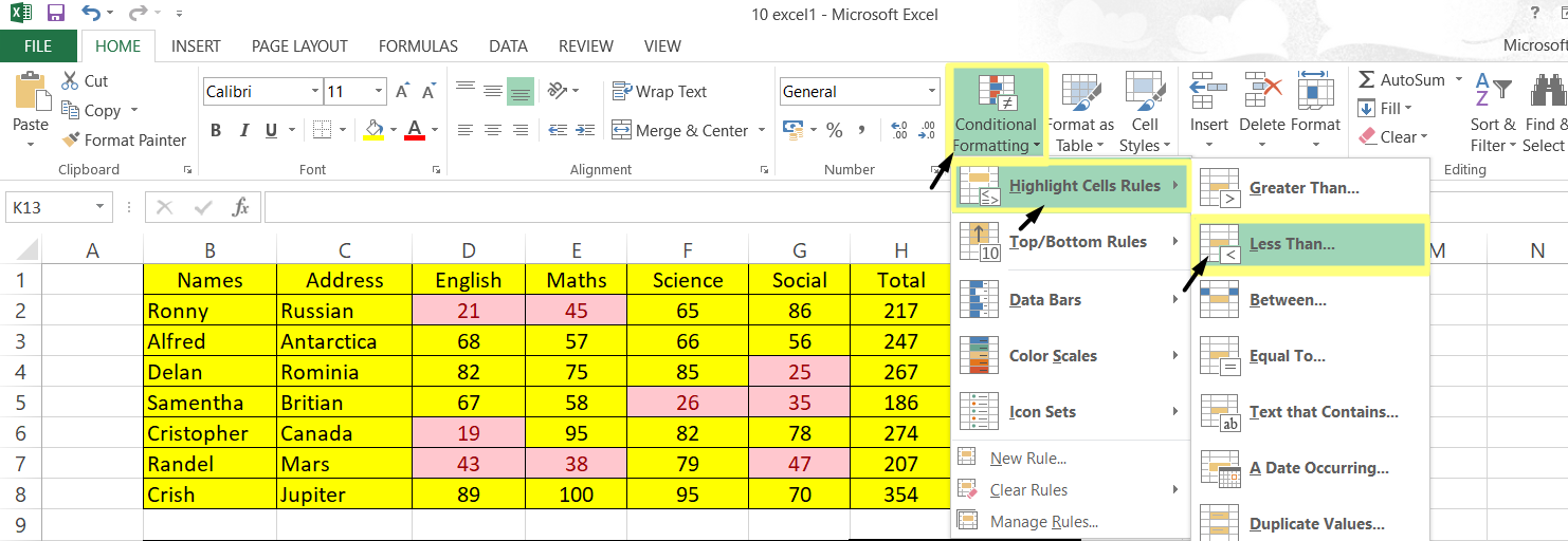

Step 4: Put the values in the pop-up then click ok.
Now the table is highlighting the marks below 50%.
10. UPPER, LOWER, TRIM.
These commands are useful when the user has huge data that is not well structured and well-formatted. All of these commands define its function. The lower feature has used to convert all the characters in small letters within a cell. The upper feature will convert all the characters in Capital letters within a cell. Trim will remove all the space within a cell.
Command keywords:
LOWER(cell_number).
UPPER(cell number).
TRIM(cell number).
Conclusion.
These are all the excel top 10 formula that everyone should know in order to boost excel skills. Each of these commands is very basic. If you want to start improving your excel skills, then you must concentrate on these basic excel top 10 formula. Each of these commands gets complex as you want to perform more complicated tasks on the excel. The importance will be more clear once you perform these formula by yourself then you will understand why we added them in the list for excel top 10 formula.
Get the best MS excel homework help from the excel homework helper. We are offering the world class excel homework assignment to the students at nominal charges.

